- PID home page »
- 5. Design and Analysis of Experiments »
- 5.8. Full factorial designs »
- 5.8.6. Assessing significance of main effects and interactions

5.8.6. Assessing significance of main effects and interactions 
When there are no replicate points, then the number of factors to estimate from a full factorial is \(2^k\) from the \(2^k\) observations. There are no degrees of freedom left to calculate the standard error or the confidence intervals for the main effects and interaction terms.
The standard error can be estimated if complete replicates are available. However, a complete replicate is onerous, because a complete replicate implies the entire experiment is repeated: system setup, running the experiment and measuring the result. Taking two samples from one actual experiment and measuring \(y\) twice is not a true replicate. That is only an estimate of the measurement error and analytical error.
Furthermore, there are better ways to spend our experimental budget than running complete replicate experiments – see the section on screening designs later on. Only later in the overall experimental procedure should we run replicate experiments as a verification step and to assess the statistical significance of effects.
There are two main ways we can determine if a main effect or interaction is significant: by using a Pareto plot or the standard error.
5.8.6.1. Pareto plot 
This is a makeshift approach that is only applicable if all the factors are centered and scaled.
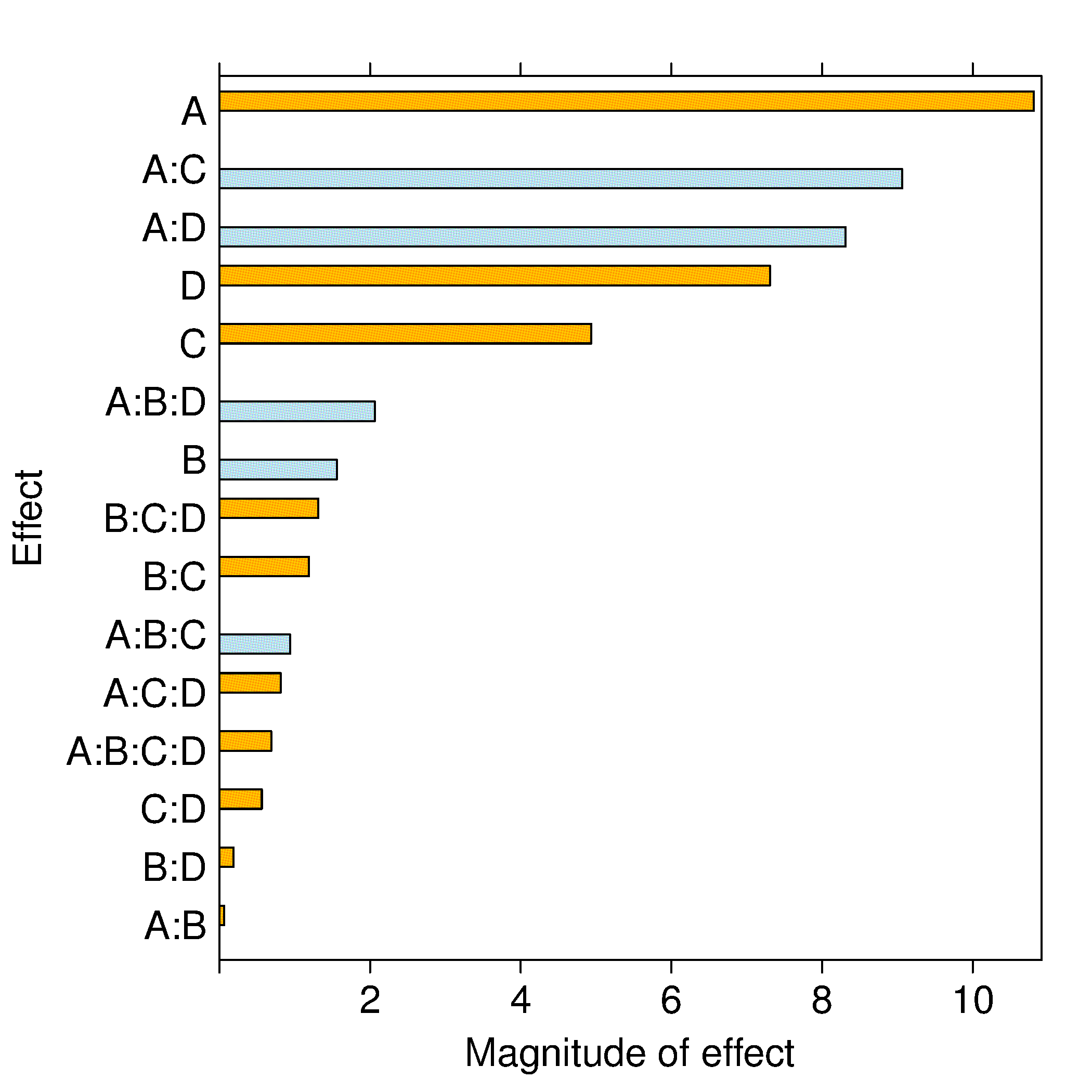
A full factorial with \(2^k\) experiments has \(2^k\) parameters to estimate. Once these parameters have been calculated, for example, by using a least squares model , then plot as shown the absolute value of the model coefficients in sorted order, from largest magnitude to smallest, ignoring the intercept term. Significant coefficients are established by visual judgement – establishing a visual cutoff by contrasting the small coefficients to the larger ones.

The example shown in the bar graph was from a full factorial experiment where the results for \(y\) in standard order were \(y = \left[45,71,48,65,68,60,80,65,43,100,45,104,75,86,70,96 \right]\) .
We would interpret that factors A , C and D , as well as the interactions of AC and AD , have a significant and causal effect on the response variable, \(y\) . The main effect of B on the response \(y\) is small, at least over the range that B was used in the experiment. Factor B can be omitted from future experimentation in this region, though it might be necessary to include it again if the system is operated at a very different point.
The reason why we can compare the coefficients this way, which is not normally the case with least squares models, is that we have both centered and scaled the factor variables. If the centering is at typical baseline operation, and the range spanned by each factor is that expected over the typical operating range, then we can fairly compare each coefficient in the bar plot. Each bar represents the influence of that term on \(y\) for a one-unit change in the factor, that is, a change over half its operating range.
Obviously, if the factors are not scaled appropriately, then this method will be error prone. However, the approximate guidance is accurate, especially when you do not have a computer or if additional information required by the other methods (discussed below) is not available. It is also the only way to estimate the effects for highly fractionated and saturated designs .

5.8.6.2. Standard error: from replicate runs or from an external dataset 
It is often better to spend your experimental budget screening for additional factors rather than replicating experiments.
If there are more experiments than parameters to be estimated, then we have extra degrees of freedom. Having degrees of freedom implies we can calculate the standard error, \(S_E\) . Once \(S_E\) has been found, we can also calculate the standard error for each model coefficient, and then confidence intervals can be constructed for each main effect and interaction. And because the model matrix is orthogonal, the confidence interval for each effect is independent of the other. This is because the general confidence interval is \(\mathcal{V}\left(\mathbf{b}\right) = \left(\mathbf{X}^T\mathbf{X}\right)^{-1}S_E^2\) , and the off-diagonal elements in \(\mathbf{X}^T\mathbf{X}\) are zero.
For an experiment with \(n\) runs, and where we have coded our \(\mathbf{X}\) matrix to contain \(-1\) and \(+1\) elements, and when the \(\mathbf{X}\) matrix is orthogonal, the standard error for coefficient \(b_i\) is \(S_E(b_i) = \sqrt{\mathcal{V}\left(b_i\right)} = \sqrt{\dfrac{S_E^2}{\sum{x_i^2}}}\) . Some examples:
A \(2^3\) factorial where every combination has been repeated will have \(n=16\) runs, so the standard error for each coefficient will be the same, at \(S_E(b_i) = \sqrt{\dfrac{S_E^2}{16}} = \dfrac{S_E}{4}\) . A \(2^3\) factorial with three additional runs at the center point would have the following least squares representation: \[\begin{split}\mathbf{y} &= \mathbf{X} \mathbf{b} + \mathbf{e}\\ \begin{bmatrix} y_1\\ y_2\\ y_3 \\ y_4 \\ y_5 \\ y_6 \\ y_7 \\ y_8 \\ y_{c,1} \\ y_{c,2} \\ y_{c,3}\end{bmatrix} &= \begin{bmatrix} 1 & A_{-} & B_{-} & C_{-} & A_{-}B_{-} & A_{-}C_{-} & B_{-}C_{-} & A_{-}B_{-}C_{-}\\ 1 & A_{+} & B_{-} & C_{-} & A_{+}B_{-} & A_{+}C_{-} & B_{-}C_{-} & A_{+}B_{-}C_{-}\\ 1 & A_{-} & B_{+} & C_{-} & A_{-}B_{+} & A_{-}C_{-} & B_{+}C_{-} & A_{-}B_{+}C_{-}\\ 1 & A_{+} & B_{+} & C_{-} & A_{+}B_{+} & A_{+}C_{-} & B_{+}C_{-} & A_{+}B_{+}C_{-}\\ 1 & A_{-} & B_{-} & C_{+} & A_{-}B_{-} & A_{-}C_{+} & B_{-}C_{+} & A_{-}B_{-}C_{+}\\ 1 & A_{+} & B_{-} & C_{+} & A_{+}B_{-} & A_{+}C_{+} & B_{-}C_{+} & A_{+}B_{-}C_{+}\\ 1 & A_{-} & B_{+} & C_{+} & A_{-}B_{+} & A_{-}C_{+} & B_{+}C_{+} & A_{-}B_{+}C_{+}\\ 1 & A_{+} & B_{+} & C_{+} & A_{+}B_{+} & A_{+}C_{+} & B_{+}C_{+} & A_{+}B_{+}C_{+}\\ 1 & 0 & 0 & 0 & 0 & 0 & 0 & 0 \\ 1 & 0 & 0 & 0 & 0 & 0 & 0 & 0 \\ 1 & 0 & 0 & 0 & 0 & 0 & 0 & 0 \end{bmatrix} \begin{bmatrix} b_0 \\ b_A \\ b_B \\ b_{C} \\ b_{AB} \\ b_{AC} \\ b_{BC} \\ b_{ABC} \end{bmatrix} + \begin{bmatrix} e_1\\ e_2\\ e_3 \\ e_4 \\ e_5 \\ e_6 \\ e_7 \\ e_8 \\ e_{c,1} \\ e_{c,2} \\ e_{c,3} \end{bmatrix}\\\end{split}\] And substituting in the values, using vector shortcut notation for \(\mathbf{y}\) and \(\mathbf{e}\) : \[\begin{split}\mathbf{y} &= \begin{bmatrix} 1 & -1 & -1 & -1 & +1 & +1 & +1 & -1\\ 1 & +1 & -1 & -1 & -1 & -1 & +1 & +1\\ 1 & -1 & +1 & -1 & -1 & +1 & -1 & +1\\ 1 & +1 & +1 & -1 & +1 & -1 & -1 & -1\\ 1 & -1 & -1 & +1 & +1 & -1 & -1 & +1\\ 1 & +1 & -1 & +1 & -1 & +1 & -1 & -1\\ 1 & -1 & +1 & +1 & -1 & -1 & +1 & -1\\ 1 & +1 & +1 & +1 & +1 & +1 & +1 & +1\\ 1 & 0 & 0 & 0 & 0 & 0 & 0 & 0\\ 1 & 0 & 0 & 0 & 0 & 0 & 0 & 0\\ 1 & 0 & 0 & 0 & 0 & 0 & 0 & 0 \end{bmatrix} \begin{bmatrix} b_0 \\ b_A \\ b_B \\ b_{C} \\ b_{AB} \\ b_{AC} \\ b_{BC} \\ b_{ABC} \end{bmatrix} + \mathbf{e}\end{split}\] Note that the center point runs do not change the orthogonality of \(\mathbf{X}\) (verify this by writing out and computing the \(\mathbf{X}^T\mathbf{X}\) matrix and observing that all off-diagonal entries are zeros). However, as we expect after having studied the section on least squares modelling , additional runs decrease the variance of the model parameters, \(\mathcal{V}(\mathbf{b})\) . In this case, there are \(n=2^3+3 = 11\) runs, so the standard error is decreased to \(S_E^2 = \dfrac{\mathbf{e}^T\mathbf{e}}{11 - 8}\) . However, the center points do not further reduce the variance of the parameters in \(\sqrt{\dfrac{S_E^2}{\sum{x_i^2}}}\) , because the denominator is still \(2^k\) ( except for the intercept term , whose variance is reduced by the center points).
Once we obtain the standard error for our system and calculate the variance of the parameters, we can multiply it by the critical \(t\) -value at the desired confidence level in order to calculate the confidence limit. However, it is customary to just report the standard error next to the coefficients, so that users can apply their own level of confidence. For example,
\[\begin{split}\text{Temperature effect}, b_T &= 11.5 \pm 0.707\\ \text{Catalyst effect}, b_K &= 1.1 \pm 0.707\end{split}\]
Even though the confidence interval of the temperature effect would be \(11.5 - c_t \times 0.707 \leq \beta_T \leq 11.5 + c_t \times 0.707\) , it is clear that at the 95% significance level, the above representation shows the temperature effect is significant, while the catalyst effect is not ( \(c_t \approx 2\) ).
5.8.6.3. Refitting the model after removing nonsignificant effects 
After having established which effects are significant, we can exclude the nonsignificant effects and increase the degrees of freedom. (We do not have to recalculate the model parameters – why?) The residuals will be nonzero now, so we can then estimate the standard error and apply all the tools from least squares modelling to assess the residuals. Plots of the residuals in experimental order, against fitted values, q-q plots and all the other assessment tools from earlier are used, as usual.
Continuing the above example, where a \(2^4\) factorial was run, the response values in standard order were \(y = [71, 61, 90, 82, 68, 61, 87, 80, 61, 50, 89, 83, 59, 51, 85, 78]\) . The significant effects were from A , B , D and BD . Now, omitting the nonsignificant effects, there are only five parameters to estimate, including the intercept, so the standard error is \(S_E^2 = \dfrac{39}{16-5} = 3.54\) , with 11 degrees of freedom. The \(S_E(b_i)\) value for all coefficients, except the intercept, is \(\sqrt{\dfrac{S_E^2}{16}} = 0.471\) , and the critical \(t\) -value at the 95% level is qt(0.975, df=11) = 2.2. So the confidence intervals can be calculated to confirm that these are indeed significant effects.
There is some circular reasoning here: postulate that one or more effects are zero and increase the degrees of freedom by removing those parameters in order to confirm the remaining effects are significant. Some general advice is to first exclude effects that are definitely small, and then retain medium-size effects in the model until you can confirm they are not significant.
5.8.6.4. Variance of estimates from the COST approach versus the factorial approach 

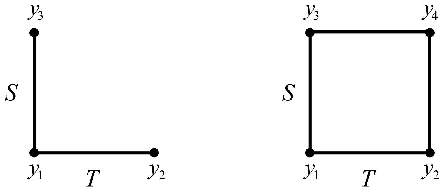
Finally, we end this section on factorials by illustrating their efficiency. Contrast the two cases: COST and the full factorial approach. For this analysis we define the main effect simply as the difference between the high and low values (normally we divide through by 2, but the results still hold). Define the variance of the measured \(y\) value as \(\sigma_y^2\) .
Not only does the factorial experiment estimate the effects with much greater precision (lower variance), but the COST approach cannot estimate the effect of interactions, which is incredibly important, especially as systems approach optima that are on ridges (see the contour plots earlier in this section for an example).
Factorial designs make each experimental observation work twice.

IMAGES
VIDEO